3 minutes
Installer InfluxDB 1.8 via Docker
Dans cet article, nous allons voir comment installer InfluxDB 1.8 et Grafana via Docker. Nous utiliserons aussi Telegraf pour vérifier que l’installation fonctionne bien.
Pour me simplifier la vie, je suis resté sur la version 1.8. La v2 est déjà disponible mais la doc étant peu fournie ou fausse, j’ai préféré ne pas me prendre la tête. (Dev perso)
Docker-compose
Créer un fichier docker-compose.yml et ajouter le contenu suivant:
Remplacer
192.168.43.5par votre IP.
version: "2"
services:
  grafana:
    image: grafana/grafana
    container_name: grafana
    restart: always
    ports:
      - 3000:3000
    networks:
      - monitoring
    volumes:
      - grafana-volume:/vol01/Docker/monitoring
  influxdb:
    image: influxdb:1.8
    container_name: influxdb
    restart: always
    ports:
      - 8086:8086
    networks:
      - monitoring
    volumes:
      - influxdb-volume:/vol01/Docker/monitoring
    environment:
      - INFLUXDB_DB=telegraf
      - INFLUXDB_USER=telegraf
      - INFLUXDB_ADMIN_ENABLED=true

      - INFLUXDB_ADMIN_USER=admin
      - INFLUXDB_ADMIN_PASSWORD=Welcome1
  telegraf:
    image: telegraf
    container_name: telegraf
    restart: always
    extra_hosts:
     - "influxdb:192.168.43.5"
    environment:
      HOST_PROC: /rootfs/proc
      HOST_SYS: /rootfs/sys
      HOST_ETC: /rootfs/etc
    volumes:
     - ./telegraf.conf:/etc/telegraf/telegraf.conf:ro
     - /var/run/docker.sock:/var/run/docker.sock:ro
     - /sys:/rootfs/sys:ro
     - /proc:/rootfs/proc:ro
     - /etc:/rootfs/etc:ro
networks:
  monitoring:
volumes:
  grafana-volume:
  influxdb-volume:
Configuration Telegraf
Créer un fichier telegraf.conf et ajouter le contenu suivant:
Une fois encore remplacer
192.168.43.5par votre IP.
[global_tags]

[agent]
  interval = "60s"
  round_interval = true
  metric_batch_size = 1000
  metric_buffer_limit = 10000
  collection_jitter = "0s"
  flush_interval = "10s"
  flush_jitter = "0s"
  precision = ""
  hostname = "192.168.43.5"
  omit_hostname = false

[[outputs.influxdb]]
urls = ["http://192.168.43.5:8086"]
database = "telegraf"
timeout = "5s"
username = "telegraf"
password = "Welcome1"


[[inputs.ping]]
interval = "5s"
urls = ["192.168.0.44", "192.168.0.131", "192.168.0.130", "google.com", "amazon.com", "github.com"]
count = 4
ping_interval = 1.0
timeout = 2.0


[[inputs.cpu]]
  percpu = true
  totalcpu = true
  collect_cpu_time = false
  report_active = false


[[inputs.disk]]
  ignore_fs = ["tmpfs", "devtmpfs", "devfs", "iso9660", "overlay", "aufs", "squashfs"]

[[inputs.diskio]]

[[inputs.kernel]]

[[inputs.mem]]

[[inputs.processes]]

[[inputs.swap]]

[[inputs.system]]
Démarrage et configuration du service
Démarrer les containers Docker avec docker-compose up.
Rendez-vous sur Grafana http://localhost:3000 et ajouter la data source “InfluxDB” contenant les données générées par Telegraf.
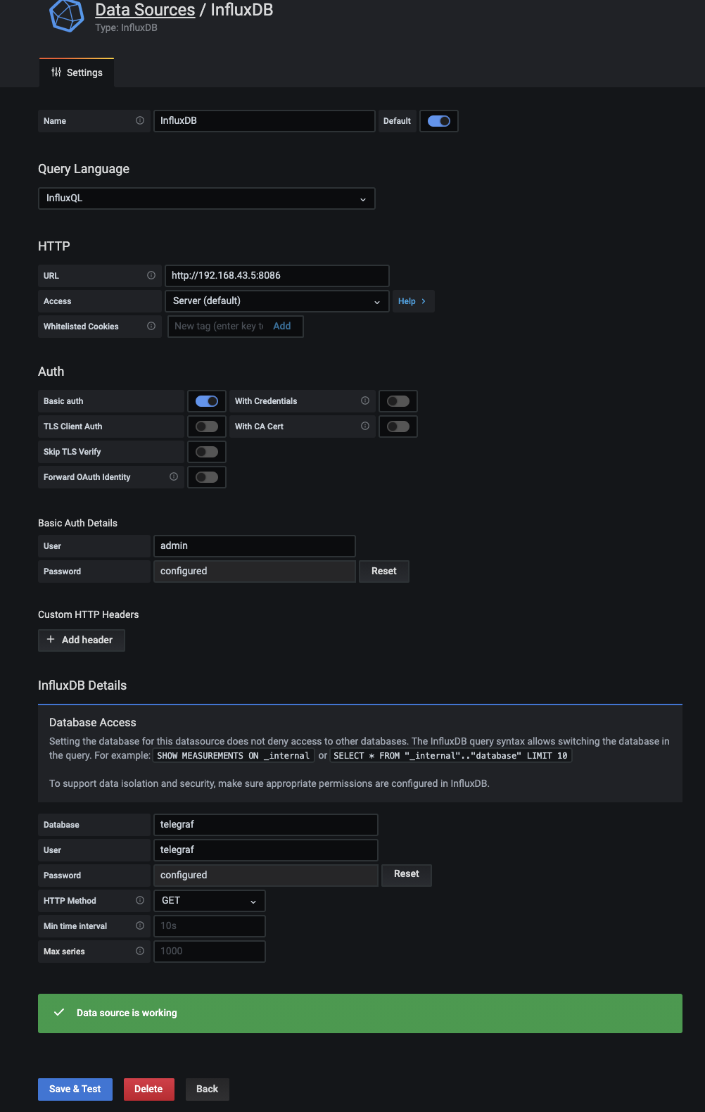
Cliquer sur “Save & Test”.
Vérification de l’existance des données
Dans un terminal, exécuter les commandes suivantes:
# Installer influxdb cli sur OSX
# brew install influxdb@1

influx
> SHOW DATABASES
> USE telegraf
> show measurements
> select * from cpu limit 5

# Output si ok
name: cpu
time                cpu       host         usage_guest usage_guest_nice usage_idle        usage_iowait         usage_irq usage_nice usage_softirq        usage_steal usage_system       usage_user
----                ---       ----         ----------- ---------------- ----------        ------------         --------- ---------- -------------        ----------- ------------       ----------
1619382480000000000 cpu-total 192.168.43.5 0           0                98.37529772028607 0.034025178632189054 0         0          0.025518883974126678 0           1.1993875467839268 0.3657706702958993
1619382480000000000 cpu0      192.168.43.5 0           0                98.43670348345952 0                    0         0          0.03398470688191586  0           1.1554800339848859 0.37383177570112885
1619382480000000000 cpu1      192.168.43.5 0           0                98.33049403741326 0.05110732538324606  0         0          0.03407155025550141  0           1.2436115843252507 0.3407155025549415
1619382540000000000 cpu-total 192.168.43.5 0           0                98.59011381006363 0.04246645150323513  0         0          0.02547987090196522  0           1.087141158483978  0.2547987090196039
1619382540000000000 cpu0      192.168.43.5 0           0                98.6591989138166  0                    0         0          0.016972165648342568 0           1.0692464358456948 0.25458248472508277
Création des Diagrammes
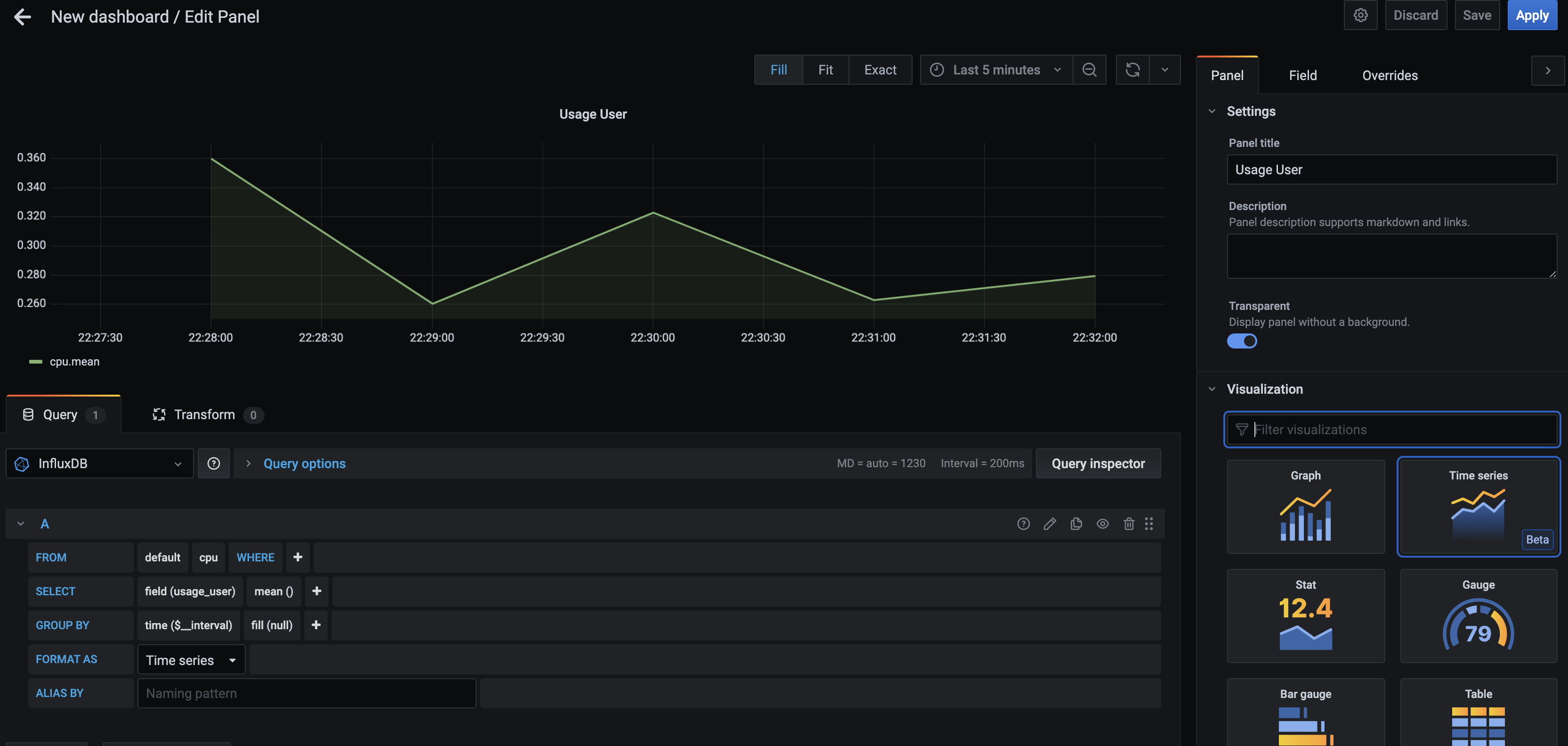
Si tout se passe bien et que vous avez des data, vous pouvez retourner sur la page d’accueil de Grafana et créer un nouveau Dashboard.
Créer ensuite un diagramme et utilisez les data Telegraf à disposition. Par exemple:
Autres diagrammes
Voilà, maintenant que vous avez vérifié que votre installation fonctionne correctement, vous pouvez créer une nouvelle DB Influx et commencer à écrire des data.
influx
> CREATE DATABASE test
> SHOW DATABASES
Exemple de code NodeJS:
Installation le package influx:
npm i --save influx. Doc officielle: https://node-influx.github.io/
const influx = new Influx.InfluxDB({
host: '192.168.43.5',
database: 'test',
port: 8086
});
/*
influx.getDatabaseNames()
.then(names => {
if (!names.include('test')) {
return influx.createDatabase('test');
}
});
*/
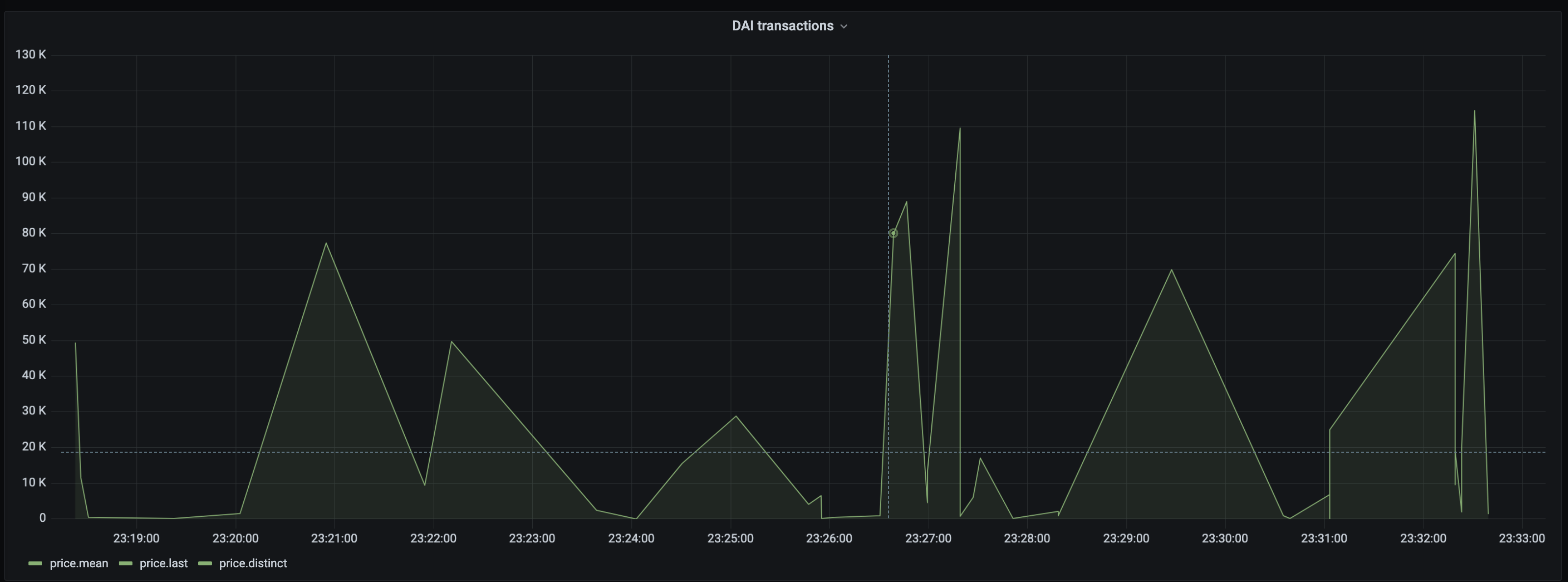
influx.writePoints([
{
measurement: 'price',
tags: { exchange: "uniswap", pool: "dai/weth" },
fields: { dai: amount, weth: 2300 }
}])
.then(() => {
console.log('Added data to the Db');
});
Et amusez vous à créer des charts. Par exemple, voici un chart (créé ultra rapidement) qui affiche les montants des transactions effectuées en DAI sur un smart contract dans la Blockchain…