Machine Learning Workflow for House Prices
Quite Practical and Far from any Theoretical Concepts 

You may be interested have a look at 10 Steps to Become a Data Scientist:
1. Machine Learning
you can Fork and Run this kernel on Github:
GitHub
I hope you find this kernel helpful and some UPVOTES would be very much appreciated
1- Introduction
This is a A Comprehensive ML Workflow for House Prices data set, it is clear that everyone in this community is familiar with house prices dataset but if you need to review your information about the dataset please visit this link.
I have tried to help Fans of Machine Learning in Kaggle how to face machine learning problems. and I think it is a great opportunity for who want to learn machine learning workflow with python completely.
I want to covere most of the methods that are implemented for house prices until 2018, you can start to learn and review your knowledge about ML with a simple dataset and try to learn and memorize the workflow for your journey in Data science world.
Before we get into the notebook, let me introduce some helpful resources.
1-1 Courses
There are a lot of Online courses that can help you develop your knowledge, here I have just listed some of them:
Machine Learning Certification by Stanford University (Coursera)
Machine Learning A-Z™: Hands-On Python & R In Data Science (Udemy)
Deep Learning Certification by Andrew Ng from deeplearning.ai (Coursera)
Python for Data Science and Machine Learning Bootcamp (Udemy))
Complete Guide to TensorFlow for Deep Learning Tutorial with Python
Data Science and Machine Learning Tutorial with Python – Hands On
- Creative Applications of Deep Learning with TensorFlow
- Neural Networks for Machine Learning
- Practical Deep Learning For Coders, Part 1
- Machine Learning
1-2 Kaggle kernels
I want to thanks Kaggle team and all of the kernel's authors who develop this huge resources for Data scientists. I have learned from The work of others and I have just listed some more important kernels that inspired my work and I've used them in this kernel:
1-3 Ebooks
So you love reading , here is 10 free machine learning books
- Probability and Statistics for Programmers
- Bayesian Reasoning and Machine Learning
- An Introduction to Statistical Learning
- Understanding Machine Learning
- A Programmer’s Guide to Data Mining
- Mining of Massive Datasets
- A Brief Introduction to Neural Networks
- Deep Learning
- Natural Language Processing with Python
- Machine Learning Yearning
I am open to your feedback for improving this kernel
2- Machine Learning Workflow
If you have already read some machine learning books. You have noticed that there are different ways to stream data into machine learning.
Most of these books share the following steps:
- Define Problem
- Specify Inputs & Outputs
- Exploratory data analysis
- Data Collection
- Data Preprocessing
- Data Cleaning
- Visualization
- Model Design, Training, and Offline Evaluation
- Model Deployment, Online Evaluation, and Monitoring
- Model Maintenance, Diagnosis, and Retraining
Of course, the same solution can not be provided for all problems, so the best way is to create a general framework and adapt it to new problem.
You can see my workflow in the below image :

Data Science has so many techniques and procedures that can confuse anyone.
2-2 Real world Application Vs Competitions
We all know that there are differences between real world problem and competition problem. The following figure that is taken from one of the courses in coursera, has partly made this comparison

As you can see, there are a lot more steps to solve in real problems.
3- Problem Definition
I think one of the important things when you start a new machine learning project is defining your problem.that means you should understand business problem.( Problem Formalization).
Problem definition has four steps that have illustrated in the picture below:

3-1 Problem Feature
We will use the house prices data set. This dataset contains information about house prices and the target value is:
- SalePrice
Why am I using House price dataset:
- This is a good project because it is so well understood.
- Attributes are numeric and categurical so you have to figure out how to load and handle data.
- It is a Regression problem, allowing you to practice with perhaps an easier type of supervised learning algorithm.
- This is a perfect competition for data science students who have completed an online course in machine learning and are looking to expand their skill set before trying a featured competition.
- Creative feature engineering .
3-1-1 Metric
Submissions are evaluated on Root-Mean-Squared-Error (RMSE) between the logarithm of the predicted value and the logarithm of the observed sales price. (Taking logs means that errors in predicting expensive houses and cheap houses will affect the result equally.)

3-2 Aim
It is our job to predict the sales price for each house. for each Id in the test set, you must predict the value of the SalePrice variable.
3-3 Variables
The variables are :
- SalePrice - the property's sale price in dollars. This is the target variable that you're trying to predict.
- MSSubClass: The building class
- MSZoning: The general zoning classification
- LotFrontage: Linear feet of street connected to property
- LotArea: Lot size in square feet
- Street: Type of road access
- Alley: Type of alley access
- LotShape: General shape of property
- LandContour: Flatness of the property
- Utilities: Type of utilities available
- LotConfig: Lot configuration
- LandSlope: Slope of property
- Neighborhood: Physical locations within Ames city limits
- Condition1: Proximity to main road or railroad
- Condition2: Proximity to main road or railroad (if a second is present)
- BldgType: Type of dwelling
- HouseStyle: Style of dwelling
- OverallQual: Overall material and finish quality
- OverallCond: Overall condition rating
- YearBuilt: Original construction date
- YearRemodAdd: Remodel date
- RoofStyle: Type of roof
- RoofMatl: Roof material
- Exterior1st: Exterior covering on house
- Exterior2nd: Exterior covering on house (if more than one material)
- MasVnrType: Masonry veneer type
- MasVnrArea: Masonry veneer area in square feet
- ExterQual: Exterior material quality
- ExterCond: Present condition of the material on the exterior
- Foundation: Type of foundation
- BsmtQual: Height of the basement
- BsmtCond: General condition of the basement
- BsmtExposure: Walkout or garden level basement walls
- BsmtFinType1: Quality of basement finished area
- BsmtFinSF1: Type 1 finished square feet
- BsmtFinType2: Quality of second finished area (if present)
- BsmtFinSF2: Type 2 finished square feet
- BsmtUnfSF: Unfinished square feet of basement area
- TotalBsmtSF: Total square feet of basement area
- Heating: Type of heating
- HeatingQC: Heating quality and condition
- CentralAir: Central air conditioning
- Electrical: Electrical system
- 1stFlrSF: First Floor square feet
- 2ndFlrSF: Second floor square feet
- LowQualFinSF: Low quality finished square feet (all floors)
- GrLivArea: Above grade (ground) living area square feet
- BsmtFullBath: Basement full bathrooms
- BsmtHalfBath: Basement half bathrooms
- FullBath: Full bathrooms above grade
- HalfBath: Half baths above grade
- Bedroom: Number of bedrooms above basement level
- Kitchen: Number of kitchens
- KitchenQual: Kitchen quality
- TotRmsAbvGrd: Total rooms above grade (does not include bathrooms)
- Functional: Home functionality rating
- Fireplaces: Number of fireplaces
- FireplaceQu: Fireplace quality
- GarageType: Garage location
- GarageYrBlt: Year garage was built
- GarageFinish: Interior finish of the garage
- GarageCars: Size of garage in car capacity
- GarageArea: Size of garage in square feet
- GarageQual: Garage quality
- GarageCond: Garage condition
- PavedDrive: Paved driveway
- WoodDeckSF: Wood deck area in square feet
- OpenPorchSF: Open porch area in square feet
- EnclosedPorch: Enclosed porch area in square feet
- 3SsnPorch: Three season porch area in square feet
- ScreenPorch: Screen porch area in square feet
- PoolArea: Pool area in square feet
- PoolQC: Pool quality
- Fence: Fence quality
- MiscFeature: Miscellaneous feature not covered in other categories
- MiscVal: Value of miscellaneous feature
- MoSold: Month Sold
- YrSold: Year Sold
- SaleType: Type of sale
- SaleCondition: Condition of sale


5-1 Import
from sklearn.linear_model import Ridge, RidgeCV, ElasticNet, LassoCV, LassoLarsCV
from sklearn.base import BaseEstimator, TransformerMixin, RegressorMixin, clone
from sklearn.linear_model import ElasticNet, Lasso,  BayesianRidge, LassoLarsIC
from sklearn.ensemble import RandomForestRegressor,  GradientBoostingRegressor
from sklearn.model_selection import KFold, cross_val_score, train_test_split
from sklearn.metrics import make_scorer, accuracy_score
from sklearn.ensemble import RandomForestClassifier
from sklearn.model_selection import cross_val_score
from sklearn.metrics import classification_report
from sklearn.model_selection import GridSearchCV
from sklearn.preprocessing import StandardScaler
from sklearn.metrics import mean_squared_error
from sklearn.preprocessing import RobustScaler
from sklearn.metrics import confusion_matrix
from sklearn.kernel_ridge import KernelRidge
from sklearn.pipeline import make_pipeline
from sklearn.metrics import accuracy_score
from sklearn.pipeline import Pipeline
import matplotlib.pyplot as plt
from scipy.stats import skew
import scipy.stats as stats
import lightgbm as lgb
import seaborn as sns
import xgboost as xgb
import pandas as pd
import numpy as np
import matplotlib
import warnings
import sklearn
import scipy
import json
import sys
import csv
import os
5-2 Version
print('matplotlib: {}'.format(matplotlib.__version__))
print('sklearn: {}'.format(sklearn.__version__))
print('scipy: {}'.format(scipy.__version__))
print('seaborn: {}'.format(sns.__version__))
print('pandas: {}'.format(pd.__version__))
print('numpy: {}'.format(np.__version__))
print('Python: {}'.format(sys.version))
pd.set_option('display.float_format', lambda x: '%.3f' % x)
sns.set(style='white', context='notebook', palette='deep')
warnings.filterwarnings('ignore')
sns.set_style('white')
%matplotlib inline
6- Exploratory Data Analysis(EDA)
In this section, you'll learn how to use graphical and numerical techniques to begin uncovering the structure of your data.
- Which variables suggest interesting relationships?
- Which observations are unusual?
By the end of the section, you'll be able to answer these questions and more, while generating graphics that are both insightful and beautiful. then We will review analytical and statistical operations:
- Data Collection
- Visualization
- Data Cleaning
- Data Preprocessing

6-1 Data Collection
Data collection is the process of gathering and measuring data, information or any variables of interest in a standardized and established manner that enables the collector to answer or test hypothesis and evaluate outcomes of the particular collection.[techopedia]
<< Note >>
The rows being the samples and the columns being attributes
# import Dataset to play with it
train = pd.read_csv('../input/train.csv')
test= pd.read_csv('../input/test.csv')
The concat function does all of the heavy lifting of performing concatenation operations along an axis. Let us create all_data.
all_data = pd.concat((train.loc[:,'MSSubClass':'SaleCondition'],
                      test.loc[:,'MSSubClass':'SaleCondition']))
<< Note 1 >>
- Each row is an observation (also known as : sample, example, instance, record)
- Each column is a feature (also known as: Predictor, attribute, Independent Variable, input, regressor, Covariate)
After loading the data via pandas, we should checkout what the content is, description and via the following:
type(train),type(test)
6-1-1 Statistical Summary
1- Dimensions of the dataset.
2- Peek at the data itself.
3- Statistical summary of all attributes.
4- Breakdown of the data by the class variable.[7]
Don’t worry, each look at the data is one command. These are useful commands that you can use again and again on future projects.
# shape
print(train.shape)
Train has one column more than test why? (yes ==>> target value)
# shape
print(test.shape)
We can get a quick idea of how many instances (rows) and how many attributes (columns) the data contains with the shape property.
You should see 1460 instances and 81 attributes for train and 1459 instances and 80 attributes for test
For getting some information about the dataset you can use info() command.
print(train.info())
if you want see the type of data and unique value of it you use following script
train['Fence'].unique()
train["Fence"].value_counts()
Copy Id for test and train data set
train_id=train['Id'].copy()
test_id=test['Id'].copy()
to check the first 5 rows of the data set, we can use head(5).
train.head(5)
1to check out last 5 row of the data set, we use tail() function
train.tail()
to pop up 5 random rows from the data set, we can use sample(5) function
train.sample(5)
To give a statistical summary about the dataset, we can use **describe()
train.describe()
To check out how many null info are on the dataset, we can use **isnull().sum()
train.isnull().sum().head(2)
train.groupby('SaleType').count()
to print dataset columns, we can use columns atribute
train.columns
type((train.columns))
<< Note 2 >> in pandas's data frame you can perform some query such as "where"
train[train['SalePrice']>700000]
6-1-2 Target Value Analysis
As you know SalePrice is our target value that we should predict it then now we take a look at it
train['SalePrice'].describe()
Flexibly plot a univariate distribution of observations.
sns.set(rc={'figure.figsize':(9,7)})
sns.distplot(train['SalePrice']);

6-1-3 Skewness vs Kurtosis
- Skewness
- It is the degree of distortion from the symmetrical bell curve or the normal distribution. It measures the lack of symmetry in data distribution. It differentiates extreme values in one versus the other tail. A symmetrical distribution will have a skewness of 0.

- It is the degree of distortion from the symmetrical bell curve or the normal distribution. It measures the lack of symmetry in data distribution. It differentiates extreme values in one versus the other tail. A symmetrical distribution will have a skewness of 0.
- Kurtosis
- Kurtosis is all about the tails of the distribution — not the peakedness or flatness. It is used to describe the extreme values in one versus the other tail. It is actually the measure of outliers present in the distribution.
#skewness and kurtosis
print("Skewness: %f" % train['SalePrice'].skew())
print("Kurtosis: %f" % train['SalePrice'].kurt())
6-2 Visualization
Data visualization is the presentation of data in a pictorial or graphical format. It enables decision makers to see analytics presented visually, so they can grasp difficult concepts or identify new patterns.
With interactive visualization, you can take the concept a step further by using technology to drill down into charts and graphs for more detail, interactively changing what data you see and how it’s processed.[SAS]
In this section I show you 11 plots with matplotlib and seaborn that is listed in the blew picture:

6-2-1 Scatter plot
Scatter plot Purpose To identify the type of relationship (if any) between two quantitative variables
# Modify the graph above by assigning each species an individual color.
columns = ['SalePrice','OverallQual','TotalBsmtSF','GrLivArea','GarageArea','FullBath','YearBuilt','YearRemodAdd']
g=sns.FacetGrid(train[columns], hue="OverallQual", size=5) \
   .map(plt.scatter, "OverallQual", "SalePrice") \
   .add_legend()
g=g.map(plt.scatter, "OverallQual", "SalePrice",edgecolor="w").add_legend();
plt.show()

6-2-2 Box
In descriptive statistics, a box plot or boxplot is a method for graphically depicting groups of numerical data through their quartiles. Box plots may also have lines extending vertically from the boxes (whiskers) indicating variability outside the upper and lower quartiles, hence the terms box-and-whisker plot and box-and-whisker diagram.[wikipedia]
data = pd.concat([train['SalePrice'], train['OverallQual']], axis=1)
f, ax = plt.subplots(figsize=(12, 8))
fig = sns.boxplot(x='OverallQual', y="SalePrice", data=data)

ax= sns.boxplot(x="OverallQual", y="SalePrice", data=train[columns])
ax= sns.stripplot(x="OverallQual", y="SalePrice", data=train[columns], jitter=True, edgecolor="gray")
plt.show()

6-2-3 Histogram
We can also create a histogram of each input variable to get an idea of the distribution.
# histograms
train.hist(figsize=(15,20))
plt.figure()

mini_train=train[columns]
f,ax=plt.subplots(1,2,figsize=(20,10))
mini_train[mini_train['SalePrice']>100000].GarageArea.plot.hist(ax=ax[0],bins=20,edgecolor='black',color='red')
ax[0].set_title('SalePrice>100000')
x1=list(range(0,85,5))
ax[0].set_xticks(x1)
mini_train[mini_train['SalePrice']<100000].GarageArea.plot.hist(ax=ax[1],color='green',bins=20,edgecolor='black')
ax[1].set_title('SalePrice<100000')
x2=list(range(0,85,5))
ax[1].set_xticks(x2)
plt.show()

mini_train[['SalePrice','OverallQual']].groupby(['OverallQual']).mean().plot.bar()

train['OverallQual'].value_counts().plot(kind="bar");

It looks like perhaps two of the input variables have a Gaussian distribution. This is useful to note as we can use algorithms that can exploit this assumption.
6-2-4 Multivariate Plots
Now we can look at the interactions between the variables.
First, let’s look at scatterplots of all pairs of attributes. This can be helpful to spot structured relationships between input variables.
# scatter plot matrix
pd.plotting.scatter_matrix(train[columns],figsize=(10,10))
plt.figure()

Note the diagonal grouping of some pairs of attributes. This suggests a high correlation and a predictable relationship.
6-2-5 violinplots
# violinplots on petal-length for each species
sns.violinplot(data=train,x="Functional", y="SalePrice")

6-2-6 pairplot
# Using seaborn pairplot to see the bivariate relation between each pair of features
sns.set()
columns = ['SalePrice','OverallQual','TotalBsmtSF','GrLivArea','GarageArea','FullBath','YearBuilt','YearRemodAdd']
sns.pairplot(train[columns],size = 2 ,kind ='scatter')
plt.show()

6-2-7 kdeplot
# seaborn's kdeplot, plots univariate or bivariate density estimates.
#Size can be changed by tweeking the value used
columns = ['SalePrice','OverallQual','TotalBsmtSF','GrLivArea','GarageArea','FullBath','YearBuilt','YearRemodAdd']
sns.FacetGrid(train[columns], hue="OverallQual", size=5).map(sns.kdeplot, "YearBuilt").add_legend()
plt.show()

6-2-8 jointplot
# Use seaborn's jointplot to make a hexagonal bin plot
#Set desired size and ratio and choose a color.
columns = ['SalePrice','OverallQual','TotalBsmtSF','GrLivArea','GarageArea','FullBath','YearBuilt','YearRemodAdd']
sns.jointplot(x="OverallQual", y="SalePrice", data=train[columns], size=10,ratio=10, kind='hex',color='green')
plt.show()

# we will use seaborn jointplot shows bivariate scatterplots and univariate histograms with Kernel density
# estimation in the same figure
columns = ['SalePrice','OverallQual','TotalBsmtSF','GrLivArea','GarageArea','FullBath','YearBuilt','YearRemodAdd']
sns.jointplot(x="SalePrice", y="YearBuilt", data=train[columns], size=6, kind='kde', color='#800000', space=0)

6-2-9 Heatmap
plt.figure(figsize=(7,4))
columns = ['SalePrice','OverallQual','TotalBsmtSF','GrLivArea','GarageArea','FullBath','YearBuilt','YearRemodAdd']
sns.heatmap(train[columns].corr(),annot=True,cmap='cubehelix_r') #draws  heatmap with input as the correlation matrix calculted by(iris.corr())
plt.show()

6-2-10 radviz
from pandas.tools.plotting import radviz
columns = ['SalePrice','OverallQual','TotalBsmtSF','GrLivArea','GarageArea','FullBath','YearBuilt','YearRemodAdd']
radviz(train[columns], "OverallQual")

6-2-12 Factorplot
sns.factorplot('OverallQual','SalePrice',hue='Functional',data=train)
plt.show()

6-3 Data Preprocessing
Data preprocessing refers to the transformations applied to our data before feeding it to the algorithm.
Data Preprocessing is a technique that is used to convert the raw data into a clean data set. In other words, whenever the data is gathered from different sources it is collected in raw format which is not feasible for the analysis. there are plenty of steps for data preprocessing and we just listed some of them :
- removing Target column (id)
- Sampling (without replacement)
- Making part of iris unbalanced and balancing (with undersampling and SMOTE)
- Introducing missing values and treating them (replacing by average values)
- Noise filtering
- Data discretization
- Normalization and standardization
- PCA analysis
- Feature selection (filter, embedded, wrapper)
6-3-1 Noise filtering (Outliers)
An outlier is a data point that is distant from other similar points. Further simplifying an outlier is an observation that lies on abnormal observation amongst the normal observations in a sample set of population.
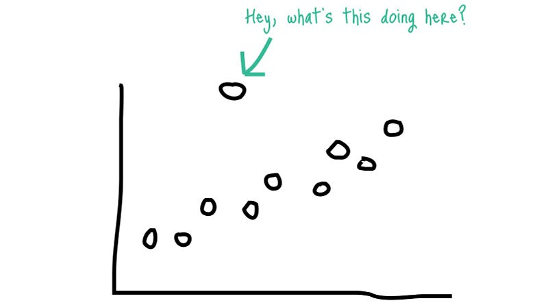 In statistics, an outlier is an observation point that is distant from other observations.
# Looking for outliers, as indicated in https://ww2.amstat.org/publications/jse/v19n3/decock.pdf
plt.scatter(train.GrLivArea, train.SalePrice, c = "blue", marker = "s")
plt.title("Looking for outliers")
plt.xlabel("GrLivArea")
plt.ylabel("SalePrice")
plt.show()

train = train[train.GrLivArea < 4000]

2 extreme outliers on the bottom right
#deleting points
train.sort_values(by = 'GrLivArea', ascending = False)[:2]
train = train.drop(train[train['Id'] == 1299].index)
train = train.drop(train[train['Id'] == 524].index)
#log transform skewed numeric features:
numeric_feats = all_data.dtypes[all_data.dtypes != "object"].index
skewed_feats = train[numeric_feats].apply(lambda x: skew(x.dropna())) #compute skewness
skewed_feats = skewed_feats[skewed_feats > 0.75]
skewed_feats = skewed_feats.index

all_data[skewed_feats] = np.log1p(all_data[skewed_feats])
all_data = pd.get_dummies(all_data)
# Log transform the target for official scoring
#The key point is to to log_transform the numeric variables since most of them are skewed.
train.SalePrice = np.log1p(train.SalePrice)
y = train.SalePrice
Taking logs means that errors in predicting expensive houses and cheap houses will affect the result equally.
plt.scatter(train.GrLivArea, train.SalePrice, c = "blue", marker = "s")
plt.title("Looking for outliers")
plt.xlabel("GrLivArea")
plt.ylabel("SalePrice")
plt.show()

6-4 Data Cleaning
When dealing with real-world data, dirty data is the norm rather than the exception. We continuously need to predict correct values, impute missing ones, and find links between various data artefacts such as schemas and records. We need to stop treating data cleaning as a piecemeal exercise (resolving different types of errors in isolation), and instead leverage all signals and resources (such as constraints, available statistics, and dictionaries) to accurately predict corrective actions.
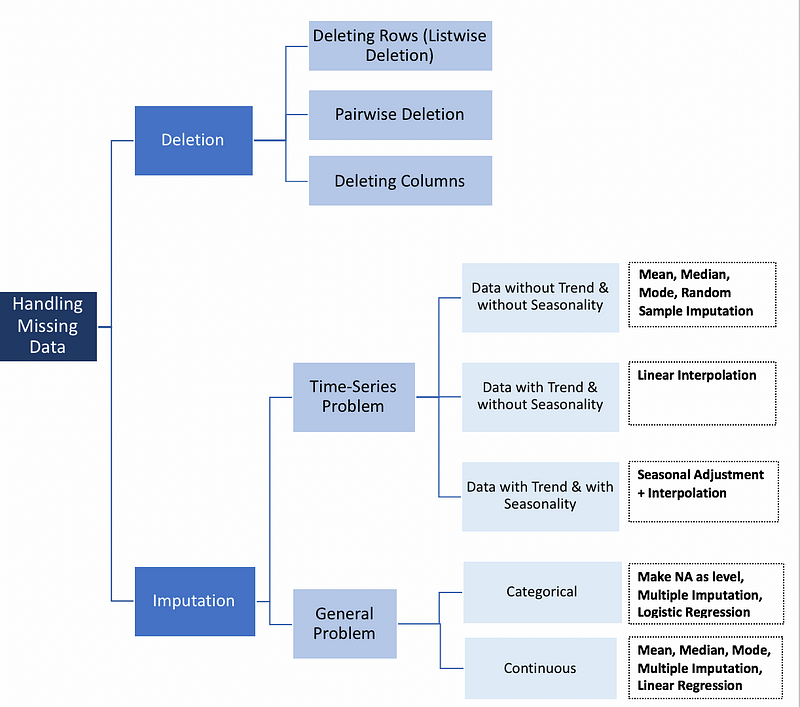
#filling NA's with the mean of the column:
all_data = all_data.fillna(all_data.mean())
7- Model Deployment
In this section have been applied plenty of learning algorithms that play an important rule in your experiences and improve your knowledge in case of ML technique.
<< Note 3 >> : The results shown here may be slightly different for your analysis because, for example, the neural network algorithms use random number generators for fixing the initial value of the weights (starting points) of the neural networks, which often result in obtaining slightly different (local minima) solutions each time you run the analysis. Also note that changing the seed for the random number generator used to create the train, test, and validation samples can change your results.
7-1 Families of ML algorithms
There are several categories for machine learning algorithms, below are some of these categories:
- Linear
- Linear Regression
- Logistic Regression
- Support Vector Machines
- Tree-Based
- Decision Tree
- Random Forest
- GBDT
- KNN
- Neural Networks
And if we want to categorize ML algorithms with the type of learning, there are below type:
Classification
- k-Nearest Neighbors
- LinearRegression
- SVM
- DT
- NN
clustering
- K-means
- HCA
- Expectation Maximization
Visualization and dimensionality reduction:
- Principal Component Analysis(PCA)
- Kernel PCA
- Locally -Linear Embedding (LLE)
- t-distributed Stochastic Neighbor Embedding (t-SNE)
Association rule learning
- Apriori
- Eclat
- Semisupervised learning
- Reinforcement Learning
- Q-learning
- Batch learning & Online learning
- Ensemble Learning
<< Note >>
Here is no method which outperforms all others for all tasks
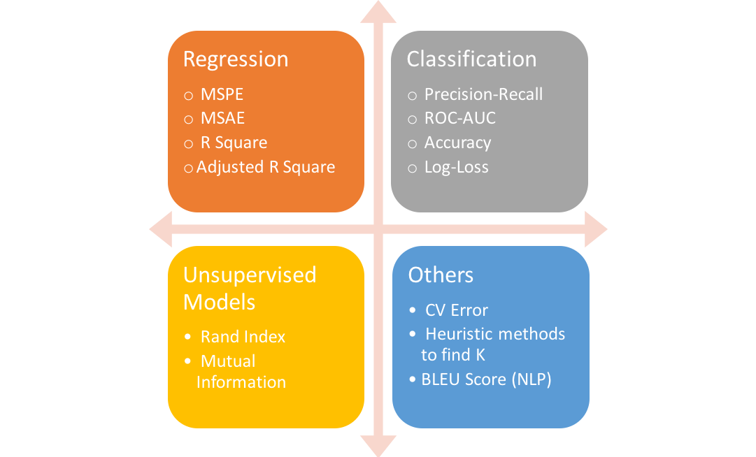
7-2 Accuracy and precision
One of the most important questions to ask as a machine learning engineer when evaluating our model is how to judge our own model?
each machine learning model is trying to solve a problem with a different objective using a different dataset and hence, it is important to understand the context before choosing a metric.
7-2-1 RMSE
Root-Mean-Squared-Error (RMSE) between the logarithm of the predicted value and the logarithm of the observed sales price. (Taking logs means that errors in predicting expensive houses and cheap houses will affect the result equally.)
#creating matrices for sklearn:
X_train = all_data[:train.shape[0]]
X_test = all_data[train.shape[0]:]
y = train.SalePrice
X_train.info()
7-3 Ridge
def rmse_cv(model):
    rmse= np.sqrt(-cross_val_score(model, X_train, y, scoring="neg_mean_squared_error", cv = 5))
    return(rmse)
model_ridge = Ridge()
alphas = [0.05, 0.1, 0.3, 1, 3, 5, 10, 15, 30, 50, 75]
cv_ridge = [rmse_cv(Ridge(alpha = alpha)).mean() for alpha in alphas]
7-3-1 Root Mean Squared Error
cv_ridge = pd.Series(cv_ridge, index = alphas)
cv_ridge.plot(title = "Validation")
plt.xlabel("alpha")
plt.ylabel("rmse")

# steps
steps = [('scaler', StandardScaler()),
         ('ridge', Ridge())]

# Create the pipeline: pipeline
pipeline = Pipeline(steps)

# Specify the hyperparameter space
parameters = {'ridge__alpha':np.logspace(-4, 0, 50)}

# Create the GridSearchCV object: cv
cv = GridSearchCV(pipeline, parameters, cv=3)

# Fit to the training set
cv.fit(X_train, y)

#predict on train set
y_pred_train=cv.predict(X_train)

# Predict test set
y_pred_test=cv.predict(X_test)

# rmse on train set
rmse = np.sqrt(mean_squared_error(y, y_pred_train))
print("Root Mean Squared Error: {}".format(rmse))
7-4 RandomForestClassifier
A random forest is a meta estimator that fits a number of decision tree classifiers on various sub-samples of the dataset and uses averaging to improve the predictive accuracy and control over-fitting. The sub-sample size is always the same as the original input sample size but the samples are drawn with replacement if bootstrap=True (default).
num_test = 0.3
X_train, X_test, y_train, y_test = train_test_split(X_train, y, test_size=num_test, random_state=100)
# Fit Random Forest on Training Set
from sklearn.ensemble import RandomForestRegressor
regressor = RandomForestRegressor(n_estimators=300, random_state=0)
regressor.fit(X_train, y_train)

# Score model
regressor.score(X_train, y_train)
7-5 XGBoost
XGBoost is one of the most popular machine learning algorithm these days. Regardless of the type of prediction task at hand; regression or classification.
7-5-1 But what makes XGBoost so popular?
Speed and performance : Originally written in C++, it is comparatively faster than other ensemble classifiers.
Core algorithm is parallelizable : Because the core XGBoost algorithm is parallelizable it can harness the power of multi-core computers. It is also parallelizable onto GPU’s and across networks of computers making it feasible to train on very large datasets as well.
Consistently outperforms other algorithm methods : It has shown better performance on a variety of machine learning benchmark datasets.
Wide variety of tuning parameters : XGBoost internally has parameters for cross-validation, regularization, user-defined objective functions, missing values, tree parameters, scikit-learn compatible API etc.[10]
XGBoost (Extreme Gradient Boosting) belongs to a family of boosting algorithms and uses the gradient boosting (GBM) framework at its core. It is an optimized distributed gradient boosting library. But wait, what is boosting? Well, keep on reading.
# Initialize model
from xgboost.sklearn import XGBRegressor
XGB_Regressor = XGBRegressor()

# Fit the model on our data
XGB_Regressor.fit(X_train, y_train)
# Score model
XGB_Regressor.score(X_train, y_train)
7-6 LassoCV
Lasso linear model with iterative fitting along a regularization path. The best model is selected by cross-validation.
lasso=LassoCV()
# Fit the model on our data
lasso.fit(X_train, y_train)
# Score model
lasso.score(X_train, y_train)
7-7 GradientBoostingRegressor
GB builds an additive model in a forward stage-wise fashion; it allows for the optimization of arbitrary differentiable loss functions. In each stage a regression tree is fit on the negative gradient of the given loss function.
boostingregressor=GradientBoostingRegressor()
# Fit the model on our data
boostingregressor.fit(X_train, y_train)
# Score model
boostingregressor.score(X_train, y_train)
7-8 DecisionTree
from sklearn.tree import DecisionTreeRegressor

# Define model. Specify a number for random_state to ensure same results each run
dt = DecisionTreeRegressor(random_state=1)
# Fit model
dt.fit(X_train, y_train)
dt.score(X_train, y_train)
7-9 ExtraTreeRegressor
from sklearn.tree import ExtraTreeRegressor

dtr = ExtraTreeRegressor()
# Fit model
dtr.fit(X_train, y_train)
# Fit model
dtr.score(X_train, y_train)
8- Conclusion
This kernel is not completed yet, I will try to cover all the parts related to the process of ML with a variety of Python packages and I know that there are still some problems then I hope to get your feedback to improve it.
Go to first step: Course Home Page
Go to next step : Titanic